Saturday, November 30, 2024

Prince的“Space”

维基百科条目链接:Space (Prince song)

这首歌所在的唱片的维基百科条目链接:Come (album)

这张专辑的全部歌曲列表链接

❀❀❀❀❀

"Space" (Universal Love Remix) 的歌词链接

"Space" (Universal Love Remix) 的音乐链接

❀❀❀❀❀

"Space"的歌词链接,下面两个版本都是这个歌词

"Space"Studio版本的音乐链接

"Space" (Acoustic Remix)的音乐链接

[Intro: NASA Sample]

T-minus sixty seconds and counting
Arm light on
Switching command to internal
Missile..Internal
Affirmative
Ready
Check
Affirmative
Affirmative

倒计时六十秒,计时开始
武器灯已开启
切换指令到内部
切换指令到内部
导弹,内部控制
确认
准备就绪
检查
确认
确认

这一段在歌曲中最后结束处再出现了一次。去过肯尼迪太空中心模拟室的人对这一段会十分熟悉。为什么会有这一段呢?象征着即将开始的激动和期待。情感的即将爆发。


[Intro]
Ooooh, oh
Ooooh, oh
Space
Ooooh

这一段前奏太美了,是Prince的歌曲的常用手法

[Verse 1]
I never been one to hide my feelings
Baby, you blow my mind
I painted your face upon my ceiling
I stare at it all the time
I imagine myself inside your bedroom
Oh, I imagine myself in your sky
You are the reason there's bass in my boom
You are the reason I'm high

我从来不会掩饰自己的感情
宝贝,你让我神魂颠倒
我把你的脸画在我的天花板上
我一直注视着它
我想象自己在你的卧室里
哦,我想象自己在你的天空中
你是我音乐中低音的原因
你让我陶醉

主歌部分描述了对爱人的迷恋。

[Pre-Chorus]
If you and I were just ten feet closer
Then I'd make you understand
That everything I wanna do to your body, baby
I would do to your hand
Then you'd be hip to the deep rush
Deeper than the boom of the bass
With every other flick of the pink plush
The closer we get to the space

如果你我再靠近十英尺
我会让你明白
我对你的身体渴望的一切,宝贝
我都会通过你的手来传达
那时你会体会到那深沉的快感
比低音的轰鸣还要深沉
每一次触碰那柔软的粉色
我们离那片空间越来越近

副歌前奏部分,描述了对爱人身体亲密的渴望。

[Chorus]
Space
Don't you want to go?
Where the souls go
Where the tears flow
Where the love grows
Do you want to go?

你不想去吗?
那里是灵魂的归宿
那里泪水流淌
那里爱意滋长
你想去吗?

副歌部分。

[Verse 2]
I never been one for this thing obsession
But just keep your eye on my hips
The circles they may be my confession
Just say the word and I'll strip
I've had dreams of us cuddling on the planet Mars
Then when I wake up, I'm all covered in sex
With eyes that fall somewhere between rubies and stars
Don't look at me, baby, or I'll flex

我从来不是那种痴迷于某件事的人。
但请注意我的臀部。
那些旋转动作或许就是我的表白。
只要你说一句话,我就会脱掉衣服。
我曾梦见我们在火星上相拥。
然后当我醒来时,我全身都充满了情欲。
你的眼神介于红宝石和星星之间。
别看我,宝贝,否则我会忍不住展示自己。

这是第二主歌

重复副歌前奏
重复副歌(稍微有一点变化)
重复NASA模拟部分
然后是结尾

[Outro]
The space...
The space...
Closer we get to the space
The space...

主歌第二部分,更是充满了对亲密关系的渴望和挑逗,表现了对方强烈的吸引力和对浪漫的梦幻,十分像描写春梦。千万不要忽略,整首歌背后都有很低沉的moans声。

❀❀❀❀❀

"Space" (Funky Stuff Remix)的歌词链接

"Space" (Funky Stuff Remix)的音乐链接

❀❀❀❀❀

Prince的12分钟长的“Come”可谓最顶级的情色歌曲,连续听几遍都不会厌倦。前面部分节奏快,铺垫和叙述,后面几分钟完全是爱欲的沉醉。远远超出Janet Jackson的Throb

Friday, November 29, 2024

标普500指数2024年第48周

2024年第48周的交易日从11月25日(周一)到11月29日(周五),但是11月28日是11月份的第四个周四,是美国的感恩节,股市关闭。11月29日周五提前到下午一点收盘,股市也在这一天收官了11月。这个周五是黑色星期五,简称“黑五”,是购物日,但是它不是股市的黑色星期五。

我们先来看看标普500指数本周的每日表现:

Date Open High Low Close Adj Close Volume
Nov 29, 2024 6,003.98 6,044.17 6,003.98 6,032.38 6,032.38 1,446,140,000
Nov 27, 2024 6,014.11 6,020.16 5,984.87 5,998.74 5,998.74 3,363,340,000
Nov 26, 2024 6,000.03 6,025.42 5,992.27 6,021.63 6,021.63 3,835,170,000
Nov 25, 2024 5,992.28 6,020.75 5,963.91 5,987.37 5,987.37 5,633,150,000
Nov 22, 2024 5,944.36 5,972.90 5,944.36 5,969.34 5,969.34 4,141,420,000

四个交易日中有三个交易日盘内创了新高,有两个交易日收盘创新高。在大约两周的震荡后,股市又开始上涨趋势。

从上表我们也可以看出,感恩节前后的交易量小很多,尤其在黑五这天。

今年至今的十一个月中,标普500指数在本月表现最出色,上涨了5.7%,主要原因就是Trump总统胜选。

值得一提的是:小型股罗素2000指数在11月上涨了10.84%,从10月31日的2,196.65升到11月29日的2,434.77,几乎触及2021年11月8日的2,442.74。

传统上来讲,小型股紧随标普500指数开启涨势才是全面牛市的特征。此时要多加小心。不过,这几年一直是科技公司带动大盘上涨,尤其是NVDA、AAPL、GOOGL、META、MSFT、NFLX、TSLA等公司,从指数上来看牛市已经很久了,但是小型股一直没有起色。到底是不是牛市?这一点在过去两年引起了很多争论。

半导体板块里面不少公司最近都有超过30%的下跌幅度,包括AMD、ASML、LRCX、MU等。不过,今天它们开始都有反转的迹象。我个人认为现在是建仓这些股票的机会。这符合我一贯的思路,当做正经生意的门槛高的公司下跌30%以上的时候,大胆上。

Sunday, November 24, 2024

标普500指数2024年第46周和第47周

2024年第46周的交易日从11月11日(周一)到11月15日(周五)。

2024年第47周的交易日从11月18日(周一)到11月22日(周五)。

我们先来看看标普500指数本周的每日表现:

Date Open High Low Close Adj Close Volume
Nov 22, 2024 5,944.36 5,972.90 5,944.36 5,969.34 5,969.34 4,141,420,000
Nov 21, 2024 5,940.58 5,963.32 5,887.26 5,948.71 5,948.71 4,230,120,000
Nov 20, 2024 5,914.34 5,920.67 5,860.56 5,917.11 5,917.11 3,772,620,000
Nov 19, 2024 5,870.05 5,923.51 5,855.29 5,916.98 5,916.98 4,036,940,000
Nov 18, 2024 5,874.17 5,908.12 5,865.95 5,893.62 5,893.62 3,983,860,000
Nov 15, 2024 5,912.79 5,915.32 5,853.01 5,870.62 5,870.62 4,590,960,000
Nov 14, 2024 5,989.68 5,993.88 5,942.28 5,949.17 5,949.17 4,184,570,000
Nov 13, 2024 5,985.75 6,008.19 5,965.91 5,985.38 5,985.38 4,220,180,000
Nov 12, 2024 6,003.60 6,009.92 5,960.08 5,983.99 5,983.99 4,243,400,000
Nov 11, 2024 6,008.86 6,017.31 5,986.69 6,001.35 6,001.35 4,333,000,000
Nov 8, 2024 5,976.76 6,012.45 5,976.76 5,995.54 5,995.54 4,666,740,000

延续第45周11月8日周五的趋势,11月11日周一盘内和收盘点数继续创新高,但是这两周标普500指数保持在小幅范围内震荡,不过,最低也只到过5,853.01而已。Trump当选效应慢慢淡了下来,市场开始回归现实。

Friday, November 22, 2024

五指湖、东方大峡谷、永不熄灭的火焰

从纽约开车返回GTA途中,我们选择在纽约州的Woodbury小镇过夜。超大的Woodbury Common Premium Outlets有两百五十家店面,我们挑选了Arc'teryx、Moose Knuckle、The North Face、Gucci、Prada、Mackage几家店逛了一遍,但是由于黑五,存货不多,最终购物无功而返。

次日上午,我们驱车前往大熊山(Bear Mountain)山顶,天气晴朗,顺利完成打卡。随后我们继续启程,发现还有时间,便计划再游览一个景点。然而,Letchworth State Park或者Eternal Flame Falls都无法在天黑前赶到,只好作罢。刚好能在落日之前抵达Ithaca,于是将目标锁定在那里。

我们直奔Ithaca Falls的Stewart Ave Historic Bridge,匆匆拍了几张照片便离开了。为了这短暂的停留,绕行了几十公里,感觉并不太值得。

Ithaca处于美国纽约州的五指湖(Finger Lakes)区域的中心地带。这片风景如画的地区值得花时间慢慢品味。即便是走马观花式的游览也至少需要三天时间。

美国纽约州的五指湖(Finger Lakes)通常指以下主要的11个湖泊,这些湖泊狭长而平行,因形似手指而得名:

  1. Seneca Lake (塞内卡湖),面积最大、最深的湖,是五指湖的核心之一。
  2. Cayuga Lake (卡尤加湖),第二大湖,最深的湖之一,著名的康奈尔大学(Cornell University)就坐落在它的东岸。
  3. Keuka Lake (库卡湖),唯一呈Y字形的湖,因独特形状被称为“五指湖中的手腕”。
  4. Canandaigua Lake (卡南代瓜湖),最西端的湖之一,以风景秀丽和高档别墅闻名。
  5. Skaneateles Lake (斯卡奈亚特雷斯湖); ,最清澈的湖之一,供给许多社区饮用水。
  6. Owasco Lake (奥瓦斯科湖),较小的湖,位于奥本市附近。
  7. Honeoye Lake (霍内奥湖),小型湖泊,以钓鱼和划船活动著称。
  8. Conesus Lake (康尼瑟斯湖),最西边的小湖,靠近罗切斯特市。
  9. Hemlock Lake (赫姆洛克湖),靠近康尼瑟斯湖,饮用水源地,周围多自然保护区。
  10. Canadice Lake (卡纳迪斯湖),五指湖中最小的一个湖泊,同样是饮用水保护区。
  11. Otisco Lake (奥蒂斯科湖),最东边的湖,面积较小,但也是五指湖系统的一部分。

点击这里可以查看五指湖区域的地图和这11个湖泊在地图上的分布。尽管统称为“五指湖”,实际上包含上述11个湖泊,而核心湖泊通常指前5个,特别是Seneca和Cayuga湖。这是文学城上的游记(1)(2)(3),值得参考。

此外,Letchwork State Park就在五指湖的西侧,距离很近,被誉为“东方大峡谷”,名气不小。游览五指湖,不会把它落下。它有上、中、下三座瀑布,游客一般从Lower falls开始逐一打卡。点击这里查看它的公园游览地图。

去了五指湖和东方大峡谷,也不要错过靠近边境的Eternal Flame Falls,欣赏大自然的奇观——永不熄灭的火焰。

大大小小的瀑布、层层叠叠的枫叶、交错如蛛网的步道,这片区域无疑值得一去再去。

Wednesday, November 20, 2024

Free Bet Blackjack 免押二十一点

除了 Bahama Bonus Blackjack,在 Fallsview Casino 还看到很多人玩 Free Bet Blackjack。

下面是 Falls View Casino 给出的 Free Bet Blackjack 的规则:


这些标准21点规则继续适用:

  • 使用六副牌
  • 庄家在软17(soft 17)需继续要牌
  • 黑杰克(Blackjack)赔率为3比2
  • 分牌后可以加倍
  • 仅限两张牌时可以加倍
  • 可重新分牌,最多分为四手,包括A对
  • 不允许投降

游戏规则变化

游戏引入了两项主要规则变化:

  1. “免费加倍”规则:
    • 当玩家的两张牌点数总和为硬9、10或11时,可以选择“免费加倍”。对于其他两张牌手牌,仍然允许普通加倍。
    • 在“免费加倍”中,庄家会用“免费筹码”匹配玩家的原始赌注,并为玩家补发一张牌。结算时:
      • 如果庄家获胜,玩家仅失去原始赌注。
      • 如果结果为平局(Push),玩家仅收回原始赌注。
      • 如果玩家获胜,玩家将收回原始赌注并获得相当于原始赌注两倍的奖金。
  2. “免费分牌”规则:
    • 玩家可以对除10点牌对以外的所有对子进行“免费分牌”。在“免费分牌”中,玩家的两张牌被分成两手单张牌手牌,原始赌注用于第一手,庄家用“免费筹码”匹配第二手的赌注。
    • 玩家可以逐手进行游戏,并在两手中都享有“免费加倍”或“免费分牌”的权利。
    • 如果玩家的手牌获胜,每个“免费筹码”将被替换为与原始赌注等额的真实筹码;如果玩家的手牌输掉或为平局,庄家将收回“免费筹码”。

庄家22点为平局

如果庄家的点数为22,而玩家的点数为21或更低,则玩家的赌注被判定为平局(Push)。

玩这个游戏的策略卡如下:

不要错过每个免费加倍和免费分牌的机会。
 

Bahama Bonus Blackjack - 西班牙21点的变种游戏

途径 Niagara Falls,天色很晚,决定在那里住下。晚上几个人去 Fallsview Casino 消磨时光。我发现标准 Blackjack 开的桌子很少,而 Bahama Bonus Blackjack、Free Bet Blackjack 和 Blackjack Switch 开的桌很多。我很久没去过赌场了,对这些新变化有些陌生。

Bahama Bonus Blackjack

下面是 Falls View Casino 给出的 Bahama Bonus Blackjack 的规则:

Bahama Bonus Blackjack

Minimums and maximums, and maximum payouts are posted at the table.

Bahama Bonus is an exciting, fast-paced version of regular Blackjack (21). Bahama Bonus is played with a deck consisting of 2, 3, 4, 5, 6, 7, 8, 9, Jack, Queen, King, & Ace…no 10’s! While basic Blackjack rules apply, it is the Match Up, Bonuses, Super Bonus and Late Surrender rules that make this game a Casino favourite.

Blackjack

Player Blackjack always beats Dealer Blackjack and pays odds of 3 to 2.

Late Surrender

If a Player is dissatisfied with their first two cards, they may surrender instead of ‘taking a hit’ or ‘standing’, thereby forfeiting half (½) of the original bet and removing themselves from the current round of play. The Player must indicate to the Dealer, their intent to surrender. Surrendering is not allowed on a Dealer Blackjack. The hand signal to surrender: place your hand palm up and move your fingers backward and forward a few times.

Pair Splitting

A Player may split cards of equal value including Aces creating up to four hands – hitting and doubling of split hands, including Aces is allowed. Bonus 21 payouts are paid on split hands. Splitting or doubling voids the Super Bonus.

Double Down

A Player may Double Down with two or more cards, on any total, even after splitting. Players may re-double up to 3 times, however the Player must double their total wager to that point and will get one additional card each time they re-double.

Double Down Rescue

If after doubling, a Player is dissatisfied with their non-busted hand, they may rescue or take back only their original wager and forfeit the doubled and re-doubled portions of their bet. A Double Down Rescue removes the Player from the current round of play.

Bonus 21 Payouts

Bahama Bonus features nine different Bonus 21 Payouts. Remember, doubling down voids all Bonus 21 Payouts.

  • 5 Card 21 Pays 3 to 2
  • 6 Card 21 Pays 2 to 1
  • 7+ Card 21 Pays 3 to 1
  • 6 - 7 - 8 Mixed Suit Pays 3 to 2
  • 6 - 7 - 8 Same Suit Pays 2 to 1
  • 6 - 7 - 8 Spades Only Pays 3 to 1
  • 7 - 7 - 7 Mixed Suit Pays 3 to 2
  • 7 - 7 - 7 Same Suit Pays 2 to 1
  • 7 - 7 - 7 Spades Only Pays 3 to 1

Super Bonus

Bahama Bonus also pays a Super Bonus of $1000 to the winner and $50 to every other betting Player! A Super Bonus occurs when the Player holds suited 7-7-7 and the Dealer’s up card is a 7 (any Suit). When a Super Bonus occurs, the Envy Bonus of $50 is paid to all other betting Players at the table, no side bet required. Splitting and doubling voids the Super Bonus.

Match Up

In addition to their regular bet, a Player can bet on the possibility that either of their first two cards will exactly match the Dealer’s up card in rank. Matches can be Suited or Non-Suited with five possible payouts.

A player makes a Bahama Bonus wager, and then places an optional second wager in the Match Up betting area. Once all bets and Match bets are made, regular play begins. The Player will receive two cards face up and the Dealer receives two cards, one face up. If either of the Player’s two cards match the Dealer’s up card, they win! All Match Up bets are settled before the start of the Bahama Bonus round.

The payouts are as follows:

    • 2 Suited Matches 24 to 1
    • 1 Non-Suited & 1 Suited Match 15 to 1
    • 1 Suited Match 12 to 1
    • 2 Non-Suited Matches 6 to 1
    • 1 Non-Suited Match 3 to 1

既然只列出了上面的一些变化,那么意味着标准21点游戏的 Dealer Hits on Soft 17 规则还继续适用。

玩这个游戏的策略卡如下(策略卡来自 Wizard of Odds 网站。):

策略卡上点名了这个是西班牙21点策略卡,因为 Bahama Bobus Blackjack 属于西班牙21点一类。

21点游戏的一副牌没有大小王,也就是52张。西班牙21点的一副牌再拿走了所有 10 的纸牌,那么就是48张。这明显不利于玩家,对庄家有利,所以增加了一些变化来弥补玩家的优势。如果玩家擅于利用这些变化,西班牙21点游戏的庄家优势比标准21点游戏低,而且没有标准21点那么死板,但是如果不会充分利用这些变化,还是去玩标准21点吧。

Wednesday, November 6, 2024

Chapter 14 Volatility Revisited

Chapter 14 Volatility Revisited

While there are many ways in which traders interpret volatility, in theory the value of an option depends on only one volatility, the volatility of the underlying contract which will occur over the life of the option. Of course, this volatility is unknown to a trader since it will occur in the future. Nevertheless, If a trader wants to use a theoretical pricing model, he will be required to make some prediction about the volatility of the underlying contract over the life of the option.

Making an Intelligent volatility forecast can be a difficult and frustrating exercise, especially for a new option trader. The forecasting of directional price movements through technical analysis is a commonly studied area in trading, and there are many sources to which a trader can turn for information on this subject. Unfortunately, volatility is a much newer concept, and there is relatively little to guide a trader. In spite of this difficulty, an option trader must make some effort to come up with a reasonable volatility input if he is going to rely on a theoretical pricing model to make intelligent trading decisions.

SOME VOLATILITY CHARACTERISTICS

The first step in making a sensible volatility forecast is to understand some of the basic characteristics of volatility. First, let's compare two graphs. Figure 14-1 shows Deutschemark prices from 1982 to 1991. Figure 14-2 shows the 50-day volatility of Deutschemarks over the same period. Are there any generalizations one can make from these graphs? Obviously both prices and volatility sometimes rise and sometimes fall. But unlike the prices of an underlying instrument, which appear to move freely in either direction, there seems to be an equilibrium number to which the volatility always returns. Over a period of three years, from early 1985 to late 1987, the price of Deutschemarks rose from a low of 29 to a high of 63. While prices fluctuated after 1987, they never reached the lows of the early 1980s. Someday, economic forces may cause Deutschemarks to rise or fall dramatically, never again returning to prices in the 50s or 60s. In other words, prices of an underlying contract are open-ended. There is no reason why they have to return to some previous level.

Such does not appear to be the case with volatility. The 50-day volatility of Deutschemarks over the 10-year period in question fluctuated from a low of 5% to a high of 20%. Yet no matter how much it fluctuated, at some point volatility always reversed itself and retraced almost all of its previous rise or fall. Indeed, we might try to find an equilibrium volatility such that there are equal fluctuations above and below this number. In the case of Deutschemarks, this equilibrium volatility seems to be about 11% to 12%. Volatility may rise well above 12%, or fall well below 11%, but eventually it always seems to return to this area.

If we were to generalize about volatility characteristics from the Deutschemark volatility in Figure 14-2, we might surmise that an underlying contract is likely to have a typical long-term average, or mean volatility. Moreover, the volatility of the underlying contract appears to be mean reverting. When volatility rises above the mean, one can be fairly certain that it will eventually fall back to its mean; when volatility falls below the mean, one can be fairly certain that it will eventually rise to its mean. There is a constant gyration back and forth through this mean.

This mean reverting characteristic of volatility can also be seen in Figure 14-3, which shows the distribution of Deutschemark volatility from 1982 to 1991. Beginning at the extreme left on the x-axis (the amount of time remaining to expiration), we can see that over any two-week period during the 10 years in question, there was a 20% chance that volatility would be either less than 6.0% or greater than 17.3% (the 10th and 90th percentiles). There was a 50% chance that volatility would be either less than 7.6% or greater than 13.0% (the 25th and 75th percentiles). The mean volatility for any two week period was 9.7%. Moving to the extreme right on the x-axis, we can see that over any 50 week period there was a 20% chance that volatility would be either less than 9.8% or greater than 14%. There was a 50% chance that volatility would be either less than 10.6% and greater than 12.7%. The mean volatility for any 50-week period was about 11.5%.

Figure 14-3 has an easily identifiable structure. As one moves further out in time the percentile lines tend to converge towards the mean, and the mean becomes stable. This reinforces the assumption that volatility is indeed mean reverting. This type of volatility graph, sometimes referred to as a volatility cone, is an effective method of presenting the volatility characteristics of an underlying instrument. (Footnote 1: For a more detailed discussion of volatility cones, see:
Burghardt, Galen and Lane, Morton; "How to Tell if Options are Cheap"; The Journal of Portfolio Management, Winter 1990, pages 72-78.)

What else can we say about volatility? Looking at the more detailed Deutschemark volatility chart in Figure 14-4, we might surmise that volatility has some trending characteristics. From July 1989 through June 1990 there was a downward trend in volatility. From July 1990 to April 1991 there was an upward trend. And from April 1991 to October 1991 there was again a downward trend. Moreover, within these major trends there were minor trends as volatility rose and fell for short periods of time.

In this respect volatility charts seem to display some of the same characteristics as price charts, and it would not be unreasonable to apply some of the same principles used in technical analysis to volatility analysis. It is important to remember, however, that while price changes and volatility are related, they are not the same thing. If a trader tries to apply exactly the same rules of technical analysis to volatility analysis, he is likely to find that in some cases the rules have no relevance, and that in other cases the rules must be modified to take into account the unique characteristics of volatility. Since the author claims no particular expertise in the area of technical analysis, the reader is left to his own devices in this regard.

VOLATILITY FORECASTING

Given the volatility characteristics that we have identified, how might we go about making a volatility forecast? First we need some volatility data. Suppose we have the following historical volatility data on a certain underlying instrument:

last 30 days 24%
last 60 days 20%
last 120 days 18%
last 250 days 18%

Certainly, we would like as much volatility data as possible. But if this is the only data available, how might we use it to make a forecast? One method might be to simply take the average volatility over the periods which we have:

(24% + 20% + 18% + 18%) / 4 = 20%

Using this method, each piece of data is given identical weight. Might it not be reasonable to assume that some data is more important than other data? A trader might assume, for example, that the more current the data, the greater its importance. Since the 24% volatility over the last 30 days is clearly more current than the other volatility data, perhaps 24% should play a greater role in our volatility forecast. We might, for example, give twice as much weight to the 30-day data as to the other data:

(40% x 24%) + (20% x 20%) + (20% x 18%) + (20% x 18%) = 20.8%

Our forecast has gone up slightly because of the extra weight given to the more recent data.

Of course, if it is true that the more recent volatility over the last 30 days is more important than the other data, it follows that the volatility over the last 60 days ought to be more important than the volatility over the last 120 days and 250 days. It also follows that the volatility over the last 120 days must be more important than the volatility over the last 250 days. We can factor this into our forecast by using a regressive weighting, giving more distant volatility data progressively less weight in our forecast.

For example, we might calculate:

(40% x 24%) + (30% x 20%) + (20% × 18%) + (10% × 18%) = 21.0%

Here we have given the 30-day volatility 40% of the weight, the 60-day volatility 30% of the weight, the 120-day volatility 20% of the weight, and the 250-day volatility 10% of the weight.

We have made the assumption that the more recent the data, the greater its importance. Is this always true? If we are interested in evaluating short term options, it may be true that data which covers short periods of time is the most important. But suppose we are interested in evaluating very long-term options. Over long periods of time the mean reverting characteristic of volatility is likely to reduce the importance of any short-term fluctuations in volatility. In fact, over very long periods of time the most reasonable volatility forecast is simply the long-term mean volatility of the instrument. Therefore the relative weight we give to the different volatility data will depend on the amount of time remaining to expiration for the options in which we are interested.

In a sense, all the historical volatility data we have at our disposal are current data; they simply cover different periods of time. How do we know which data is the most important? In addition to the mean reverting characteristic, volatility also tends to exhibit serial correlation. The volatility over any given period is likely to depend on, or correlate with, the volatility over the previous period, assuming that both periods cover the same amount of time. If the volatility of a contract over the last four weeks was 15%, the volatility over the next four weeks is more likely to be close to 15% than far away from 15%. We can again use the weather analogy from Chapter 4. If the high temperature yesterday was 25°, and we had to guess what the high temperature today would be, a guess of 30° would make more sense than a guess of 50°. Once we realize this, we might logically choose to give the greatest weight to the volatility data covering a time period closest to the life of the options in which we are interested. That is, if we are trading very long-term options, the long-term data should get the most weight. If we are trading very short term options, the short term data should get the most weight. And if we are trading intermediate-term options, the intermediate-term data should get the most weight.

Suppose we are interested in evaluating six-month options. How should we weight our data? Since 120 (trading) days is closest to six months, we can give the 120-day data the greatest weight, and give other data correspondingly lesser weight:

(15% × 24%) + (25% x 20%) + (35% x 18%) + (25% × 18%) = 19.4%

Alternatively, if we are interested in 10-week options, we can give the greatest weight to the 60-day volatility data:

(25% x 24%) + (35% x 20%) + (25% x 18%) + (15% × 18%) = 20.2%

In the foregoing examples we used only four historical volatilities, but the more volatility data which is available, the more accurate any volatility forecast is likely to be. Not only will more data, covering different periods of time, give a better overview of the volatility characteristics of an underlying instrument, but it will enable a trader to more closely match historical volatilities to options with different amounts of time to expiration. In our example we used historical volatilities over the last 60 days and 120 days as approximations to forecast volatilities for six-month and 10-week options. Ideally, we would like historical data covering exactly a six-month period and exactly a 10-week period.

The method we have described is one which many traders intuitively use to forecast volatility. It depends on identifying the typical characteristics of volatility, and then projecting a volatility over the forecasting period. Theoreticians have recently tried to take essentially the same approach to volatility forecasting, and this has led to the development of autoregressive conditional heteroskedasticity (ARCH) and generalized autoregressive conditional heterosexuality (GARCH) volatility models. A detailed discussion of such models is beyond the scope of this text, since they can be mathematically complex and are not widely used among traders. Nevertheless, an option trader should be aware that these models do exist, and that they are simply an attempt to apply the mean reverting and serial correlation characteristics of volatility to volatility forecasting. (Footnote 2: For further information on ARCH and GARCH models see:
Engie, R.F., "Autoregressive Conditional Heteroskedaticity with Estimates of the Varlance of United Kingdom Inflation," Econometrica, Vol. 50, No. 4, 982, pages 987-1000.
Bollerslev, T., "Generalized Autoregressive Conditional Heteroskedasticity," Journal of Economics, No. 31, April 1986, pages 307-327.
Bollerslev, T., "A Conditional Heteroskedastic Time Serles Model for Speculative Prices and Rates of Return," Revtew of Economics and Statistics, No. 69, August 1987, pages 542-547.
Nelson, David B., "Conditional Heteroskedasticity in Asset Returns: A New Approach," Econometrica, No. 59, 1991, pages 347-370
Kuberek, Robert C., "Predicting Interest Rate Volatility: A Conditional Heteroskedastic Model of Interest Rate Movements," Journal of Fixed Income, Vol. 1, No. 4, March 1992, pages 21-27.)

Thus far we have focused only on the historical volatility characteristics of the underlying instrument in trying to forecast a volatility. Is there any other information which might be useful? No individual trader can hope to know everything affecting price changes in an underlying contract. Perhaps there are factors which could affect the future volatility, but about which the trader is unaware. If one believes that such information is likely to be reflected in the prices of the contracts being traded, one way to ferret out additional volatility information is to look at the prices of options. In other words, a trader will want to look at the implied volatility in the marketplace to find the consensus volatility. Once he has done this, he will want to use this information in any volatility forecast he intends to make.

How much weight should a trader give the implied volatility? Some traders subscribe to the efficient market principle, and believe that the implied volatility is always the best volatility forecast since it reflects all available information. Most traders believe, however, that while the implied volatility is important, it isn't the whole story. Typically, a trader might give the implied volatility a weighting somewhere between 25% and 75% in making a volatility forecast. How much depends on the trader's confidence in forecasting a volatility based on historical volatility data? If a trader feels very confident about his forecast, he might give the implied volatility as little as a 25% weight; if he feels uncertain about his forecast, he might give the implied volatility as much as a 75% weight. Of course, his confidence level will depend on his experience, as well as how conclusive the historical data is.

For example, suppose a trader has made a volatility forecast of 20% based on historical data, and that the implied volatility is currently 24%. If the trader decides to give the implied volatility 75% of the weight, his final forecast will be:

(75% x 24%) + (25% × 20%) = 23%

On the other hand, if the trader decides to give the implied volatility 25% of the weight, his final forecast will be:

(25% x 24%) + (75% x 20%) = 21%

Finally, If the trader decides to give the implied volatility half the weight, his final forecast will be:

(50% × 24) + (50% × 20) = 22%

A PRACTICAL APPROACH

No matter how painstaking a trader's method, he is likely to find that his volatility forecasts are often incorrect, and sometimes to a large degree. Given this difficulty, many traders find it easier to take a more general approach. Rather than asking what the correct volatility is, a trader might instead ask, given the current volatility climate, what's the right strategy? Rather than trying to forecast an exact volatility, a trader will try to pick a strategy that best fits the volatility conditions in the marketplace. To do this, a trader will want to consider several factors:

  1. What is the long-term mean volatility of the underlying contract?
  2. What has been the recent historical volatility in relation to the mean volatility?
  3. What is the trend in the recent historical volatility?
  4. Where is implied volatility and what is its trend?
  5. Are we dealing with options of shorter or longer duration?
  6. How stable does the volatility tend to be?

For example, suppose there are ten weeks (approximately 50 trading days) to expiration and we are trying to decide on an appropriate volatility strategy. To make a decision, we might look at the 50-day historical volatility (the historical volatility which corresponds to the amount of time remaining to expiration), its relationship to the long-term mean volatility, and of course the implied volatility. Having done this, suppose we find the conditions shown in Figure 14-5A. What are our conclusions?

Clearly we are coming off a period of high volatility and seem to be moving downward. The recent 50-day historical volatility (approx. 20.6%) is still above the long-term historical mean (approx. 18.7%), so there is reason to believe that the volatility will continue to decline. The implied volatility is also declining, but still appears to be about 1½ percentage points higher (22.1%) than the 50-day historical volatility. All volatility conditions seem to be pointing in the same direction. The historical volatility is above the mean but declining, and the implied volatility is above the historical volatility and also declining. A short volatility position (negative gamma/negative vega) is strongly indicated.

There are of course a variety of short volatility strategies available, and the best strategy will still depend on a trader's experience in the market and the amount of risk he is willing to take. Suppose we have additional volatility data (perhaps a volatility cone of the type in Figure 14-3) showing that the 50-day volatility can easily vary by as much as 10 percentage points. We still want to sell volatility, but given this instability and the fact that implied volatility at 22.2% is only slightly above the 50-day historical volatility, perhaps the wisest choice is a less risky strategy such as the purchase of butterflies. If a riskier strategy is chosen, perhaps it should be done only in small size. On the other hand, if implied volatility is currently 25% and we find that the volatility tends to be quite stable, varying only five or six percentage points for any 50-day period, a trader may be willing to take on a much riskier position, perhaps selling a straddles or strangles.

In real life the situation is rarely as simple as in Figure 14-5A. For example, consider Figure 14-5B. Now the historical volatility is above the historical mean and declining, but the implied volatility has already moved ahead of the historical volatility. A trader may still choose a short volatility position, but he is unlikely to have the same degree of confidence. Indeed, the situation may be even more confused. Suppose the historical volatility is above the long-term mean but seems to be increasing (Figure 14-5C). Or suppose implied volatility is moving in the opposite direction of the historical volatility (Figure 14-5D). In each of these situations some factors dictate one type of position, while other factors dictate a different position.

Consider the situation in Figure 14-6A where we are thinking of taking a position in six-week options (approximately 30 trading days). The 30-day historical volatility, currently at 15.8%, is well above the long-term mean of 11.2%. However, the trend in volatility seems to be up, and there is no telling how long it will take for the volatility to revert to its mean of 11.2%. The current Implied volatility of 14.6% is also well above the long term mean volatility, but is lower than the 30-day historical volatility. Corresponding to the upward trend in historical volatility, there also seems to be an upward trend in the implied volatility. With so many contradictory signals, a trader is unlikely to have a strong opinion about whether he should buy or sell volatility. He may choose to take no position at all, preferring to wait for clearer indications.

Suppose, in addition to six-week options, we also have available 19-week options (approximately 95 trading days). Volatility data for this contract is shown in Figure 14-6B. While a trader may be hesitant to take a position in six-week options alone, when combined with 19-week options, he may be able to construct a strategy with much more acceptable risk characteristics. Here the 95-day historical volatility of 12.6% is above the 11.2% mean volatility. Moreover the current implied volatility of 19-week options, at 14.5%, is well above both the 95-day historical volatility and the long-term mean volatility. There is a much better chance that the volatility will revert to its mean over a 19-week period than over a six-week period, so there are much stronger reasons for taking a short volatility position in 19 week options than in six-week options. Still, the upward trend in both the historical and implied volatilities will cause some worry if we do take a short volatility position. However, If we were to simultaneously take a long volatility position in six-week options, we would at least be protected against a continuing increase in the volatility of the underlying contract over the next six weeks. By creating a short time spread (buy six-week options/ sell 19-week options) we can take a position which should be profitable based on our knowledge of volatility characteristics, but which also has acceptable risk characteristics if we are wrong.

A short time spread will not eliminate every risk. The market might suddenly become very quiet, with historical volatility quickly dropping to, or even below, its long-term mean. At the same time, implied volatility may remain relatively high. Such conditions will do the most damage to a short time spread. Still, if we believe that the implied volatility tends to follow the historical volatility, we may conclude that it is unlikely that the implied volatility will stay high if the historical volatility drops.

A trader will always attempt to pick the strategy which best fits his opinion of market conditions, whether a directional opinion or a volatility opinion. Given the fact that there is such a wide variety of market conditions, a trader who is familiar with the greatest number of strategies will have the best chance of surviving and prospering. He will be in a position to pick strategies with the best risk/ reward characteristics, strategies which will be profitable when things go right, but which won't give back all the profits when things go wrong. This skill comes not only from a technical knowledge of option evaluation and theory, but also from a practical knowledge of what really happens in the marketplace.

SOME THOUGHTS ON IMPLIED VOLATILITY

Since many option strategies are sensitive to changes in implied volatility, and since implied volatility will often play a role in forecasting the volatility of the underlying contract, it may be worthwhile to consider some of the characteristics of implied volatility.

Implied versus Historical Volatility

Implied volatility can be thought of as a consensus volatility among all market participants with respect to the expected amount of underlying price fluctuation over the remaining life of an option. In the same way that an individual trader is likely to change his volatility forecast in response to changing historical volatility, it is logical to assume that the marketplace as a whole will also change its consensus volatility in response to changing historical volatility. As the market becomes more volatile, implied volatility can be expected to rise; as the market becomes less volatile, implied volatility can be expected to fall, Market participants are making the logical assumption that what has happened in the past is a good indicator of what will happen in the future.

The influence of historical volatility on implied volatility can be seen in Figure 14-7, the historical and implied volatility of U.S. Treasury Bond futures traded on the Chicago Board of Trade from 1989 to 1991. In late 1989, and again in mid-1991, there were declines in the volatility of Treasury Bond futures, and these were accompanied by corresponding declines in implied volatility. From August 1990 through January 1991 (the period of the Iraqi invasion of Kuwait), there were several sharp increases in the volatility of the futures, and these were accompanied by similar increases in implied volatility. Clearly, the marketplace, in the form of changing implied volatility, was responding to the changing historical volatility of the underlying contract.

Notice, however, that the fluctuations in implied volatility were usually less than the fluctuations in historical volatility. When the historical volatility declined, the implied volatility rarely declined by an equal amount. And when historical volatility increased, the implied volatility rarely increased by an equal amount. Because volatility tends to be mean reverting, when historical volatility is above its mean there is a greater likelihood that it will decline, and when historical volatility is below its mean there is a greater likelihood that it will increase.

Moreover, the further out in time we go, the greater the likelihood that the volatility of the underlying contract will return to its mean. (Look again at Figure 14-3.) Consequently, the implied volatility of long-term options tends to remain closer to the mean volatility of an underlying contract than the implied volatility of short-term options. As historical volatility rises, the implied volatility of all options is likely to rise. But given the stronger mean reverting characteristics of volatility over long periods of time, the implied volatility of long-term options will tend to rise less than the implied volatility of short-term options. As historical volatility falls, the implied volatility of all options is likely to fall. But the implied volatility of long-term options will tend to fall less than the implied volatility of short-term options. This is born out by Figure 14-8, the implied volatility of Treasury Bond options for various expiration months from September 1990 to May 1991. Note the increase in implied volatilities during January 1991. But the increase in the implied volatility of the short term contract (March) was much greater than the increase in the implied volatility of the mid-term (June) contract, which was in turn greater than the increase in the implied volatility of the long-term (September) contract. When implied volatility began to decline in late January 1991 the roles were reversed. The March contract declined the most rapidly, followed by the June contract, and the September contract. This is typical of the way in which implied volatility tends to change in response to changing volatility environments.

Over long periods of time the historical volatility of the underlying contract will be the dominant factor affecting implied volatility. Over short periods of time, however, other factors can also play a significant, perhaps even a dominant, role. If the marketplace foresees events which could cause the underlying contract to become more volatile, anticipation of these events might cause implied volatility to change in ways that are not necessarily consistent with historical volatility. For example, government reports on economic conditions are issued periodically, and these reports have been known to contain surprises for the interest rate and foreign exchange market. This potential for surprise can cause uncertainty in the marketplace, and this uncertainty is often reflected in an increase in implied volatility. Going into government reports, there is a strong tendency for implied volatility to rise, even in the face of low historical volatility in the underlying instrument.

Government reports are not the only factors which add uncertainty to the market. Any future events which could have unexpected consequences can have an effect on Implied volatility. In the currency markets, upcoming meetings of finance ministers-or in the energy markets upcoming OPEC meetings— often cause implied volatility to rise. In the stock option market, earnings news, the potential success or failure of new products, or (most dramatically) the possibility of a takeover, can all cause increases in implied volatility, regardless of the historical volatility of the stock.

In a similar way, if the marketplace believes that no significant events are likely to occur in the foreseeable future, uncertainty is removed from the market. In such a case the implied volatility may start to fall, even if the actual historical volatility has been relatively high. This is why implied volatility sometimes drops right after large moves in the underlying contract. Once the big event has occurred, there may be a perception that all the uncertainty has been removed from the market.

Regardless of short-term changes in implied volatility, it is still important for a trader to remember that the volatility of the underlying contract will eventually overwhelm any considerations of implied volatility. As an example, consider the following situation:

futures price = 97.73
time to expiration = 60 days
interest rate = 6%
implied volatility = 20%

Given these conditions, the 100 call would be trading for 2.17, with an implied delta of 40. Suppose we create a delta neutral position by purchasing ten 100 calls for 2.17 each, and selling four futures contracts at 97.73. What will happen to our position if implied volatility rises to 22%?

If implied volatility immediately goes to 22%, the new price of the 100 call will be 2.47, and we will show a profit of

10 × (2.47 - 2.17) = +3.00

Suppose, however, that the increase in implied volatility occurs very slowly, over a period of 20 days, and during this period the price of the underlying futures contract remains at 97.73. Under these conditions, even if implied volatility rises from 20% to 22%, the 100 call will now be worth only 1.87. Our position will then show a loss of

10 × (1.87 - 2.17) = -3.00

Even though the implied volatility increased, the fact that the underlying futures contract failed to make any significant move resulted in the option's price declining.

Now suppose we have the same position (long ten 100 calls, short four futures contracts) but this time instead of rising to 22%, the implied volatility drops to 18%. What will be the effect on our position?

If implied volatility immediately drops to 18%, the new price of the 100 call will be 1.86, and we will show a loss of

10 × (1.86 - 2.17) = -3.10

Suppose, however, that the decline in implied volatility is accompanied by a swift move in the underlying contract. If the underlying futures contract falls to 93.00, and implied volatility falls to 18%, the price of the 100 call will be .59, and we will show a profit of 4 × (97.73 - 93.00) - 10 × (2.17 - 59) = +3.12

On the other hand, if the underlying futures contract rises to 102.50 while implied volatility falls to 18%, the price of the 100 call will be 4.32, and we will again show a profit

4 × (97.73 - 102.50) + 10 × (4.32 - 2.17) = +2.42

In both cases the movement in the underlying contract has more than offset any decline in the option's price due to a decline in implied volatility.

The foregoing examples are of course simplified. As market conditions change-an active trader may very well make adjustments to his position in order to remain delta neutral. If so, the actual profit or loss will be affected by the cash flow from this adjustment process. The important point is that the volatility of the underlying contract, whether the contract moves or sits still over time, will eventually overwhelm any changes in implied volatility. This is not to say that implied volatility is unimportant. The price of a contract is always an important consideration in making trading decisions. But in order to trade intelligently, we need to know value as well as price. The value of an option is determined by the volatility of the underlying contract over the life of the option.

Implied versus Future Volatility

If, as many traders believe, prices in the marketplace reflect all available information affecting the value of a contract, the best predictor of the future volatility ought to be the implied volatility. Just how good a predictor of future volatility is implied volatility? While it would be impossible to answer this question definitively, since that would require a detailed study of many markets over long periods of time, we might still gain some insight by looking at a limited number of examples.

Clearly, no one knows the future volatility. We can, however, record the implied volatility at any moment in time and then, when expiration arrives, look back and calculate the actual volatility of the underlying contract between the time we recorded the implied volatility and expiration. We can do this every day during an option's life, recording the implied volatility and then at expiration calculating the actual volatility that occurred over this period. This has been done in Figures 14-9A, 9B, and 9C for the June 1992, March 1993, and December 1993 options on Treasury Bond futures. It is admittedly dangerous to generalize from such limited data, but are there any conclusions we might draw from these graphs?

We can see that with a great deal of time remaining to expiration, the future volatility of the underlying contract (the solid line) is relatively stable. But as we get closer to expiration the future volatility can become much less stable. This is logical if we again recall that the mean reverting characteristics of volatility are much less certain over short periods of time than over long periods. One large move in the underlying contract with only several days remaining to expiration will result in a sharp increase in the volatility to expiration (see Figure 14-9C). On the other hand, if the underlying contract is relatively quiet over the last several days in an option's life, the volatility to expiration will collapse (see Figure 14-9B).

How does the marketplace react to these volatility characteristics? With long periods of time remaining to expiration, the volatility to expiration is relatively stable. One would therefore expect the implied volatility to also be relatively stable. Conversely, with short periods of time remaining to expiration, the volatility to expiration can be very unstable, and one would therefore expect the implied volatility to be unstable. These conclusions are born out by the implied volatility (the broken line) in Figures 14-9A, 9B, and 9C. Over long periods of time, the marketplace is reacting to many events. This is easier than reacting to a limited number of events, which is what the marketplace is faced with over a short period of time. The marketplace knows that the laws of probability are more likely to balance out over many occurrences than over only a few occurrences.

Note also that there is no guarantee that the marketplace will have the correct implied volatility. The implied volatility is a guess, and guesses carry with them the possibility of error, sometimes very large error. In Figure 14-9B the implied volatility turned out to be much too high over almost all of the option's life. Had a trader sold premium at any time, he would have shown a profit. At its most extreme, during October 1992, there was almost a four percentage-point difference between the implied volatility of the March 1993 options and the future volatility of the March 1993 futures contract. In Figure 14-9C the implied volatility was too high during the early part of the option's life, but too low during the latter part. During the few weeks prior to expiration, the implied volatility was too low by as much as three percentage points. Finally, in Figure 14-9A the implied volatility was relatively accurate over the early part of the option's life, but too high during the latter part.

It should be clear by now that dealing with volatility is a difficult task. To facilitate the decision-making process we have attempted to make some generalizations about volatility characteristics. Even then, if one decides to become involved in a market it may not be at all clear what the right strategy is. Moreover, we have looked at a limited number of examples, making the generalizations even less reliable. Every market has its own characteristics, and knowing the volatility characteristics of a particular market, whether interest rates, foreign currencies, stocks, or a physical commodity, is at least as important as knowing the technical characteristics of volatility. And this knowledge can only come from careful study of a market combined with actual trading experience.

Chapter 13 Hedging with Options

Chapter 13 Hedging with Options
第十三章 使用期权进行对冲

The original justification for introducing options and futures was to enable market participants to transfer part or all of the risk associated with holding a position in the underlying instrument from one party to another. Options and futures act as insurance contracts. Unlike a futures contract, an option transfers only part of the risk from one party to another. In this respect an option acts much more like a traditional insurance policy than a futures contract.

期权和期货的最初引入是为了让市场参与者能够将持有标的资产的部分或全部风险转移给他人。期权和期货的作用类似于保险合约。但与期货合约不同,期权只转移部分风险,因此期权更像传统的保险单,而非期货合约。

Even though options were originally intended to function as insurance policies, option markets have evolved to the point where, in most markets, hedgers (those wanting to protect an existing position), make up only a small portion of market participants. Other traders, including arbitrageurs, speculators, and spreaders, typically outnumber true hedgers. Nevertheless, hedgers still represent an important force in the marketplace, and any sophisticated market participant must be aware of the strategies hedgers use to protect their positions.

尽管期权的初衷是作为保险工具,期权市场已经发展到如今,在大多数市场中,对冲者(即想保护现有头寸的参与者)仅占少部分。其他交易者,如套利者、投机者和价差交易者,通常数量多于真正的对冲者。尽管如此,对冲者在市场中仍然是重要力量,任何有经验的市场参与者都需要了解对冲者保护头寸的策略。

Many hedgers come to the marketplace as either natural longs or natural shorts. Through the course of normal business activities they will profit from either a rise or fall in the price of some underlying Instrument. The producer of a commodity (grain, oil, precious metals) is a natural long; if the price of the commodity rises, he will receive more when he goes to sell it in the marketplace. The user of a commodity is a natural short; if the price of the commodity falls, he will have to pay less for it when he goes to buy it in the marketplace. In the same way, lenders and borrowers in the financial markets are natural longs and shorts in terms of interest rates. A rise in interest rates will help lenders and hurt borrowers. A decline in interest rates will have the opposite effect.

许多对冲者进入市场时就带有天然的多头或空头属性。在正常业务活动中,他们会因某些标的资产价格的上涨或下跌而获利。例如,大宗商品(如谷物、石油、贵金属)的生产者是天然多头,如果商品价格上涨,他在市场上销售时会获得更多收入。商品的使用者则是天然空头,如果商品价格下跌,他在购买时的支出会减少。同样,在金融市场中,借贷双方在利率方面也具有天然的多头和空头属性。利率上升有利于贷方而不利于借方,利率下降则反之。

Other potential hedgers come to the marketplace because they have voluntarily chosen to take long or short positions, and now wish to lay off part or all of the risk of that position. A speculator may have taken a long or short position in a certain contract, but wishes to temporarily reduce the risk associated with an outright long or short position. For example, a portfolio manager is usually paid to choose which stocks to buy for a portfolio. He is a voluntary long. If he wants to continue to hold certain stocks, but believes that the stocks might decline in the short term, he may find it cheaper to temporarily hedge the stocks with options or futures than to sell the stocks and buy them back at a later date.

其他潜在对冲者进入市场的原因是主动选择了多头或空头头寸,现在希望转移部分或全部风险。投机者可能建立了某合约的多头或空头头寸,但希望暂时减少此类头寸的风险。例如,投资组合经理通常负责为投资组合选择股票,是自愿的多头。如果他想继续持有某些股票,但认为短期内可能下跌,他可能发现用期权或期货对冲这些股票的成本比卖出后再买入更低。

As with insurance, there is a cost to hedging. The cost may be immediately apparent because it requires an immediate cash outlay. But the cost may also be more subtle, either in terms of lost profit opportunity, or in terms of additional risk under some circumstances. Every hedging decision is a tradeoff: what is the hedger willing to give up under one set of market conditions in order to protect himself under another set? A hedger with a long position who wants to protect his downside will almost certainly have to give up something on the upside; a hedger with a short position trying to protect his upside will have to give up something on the downside.

如同保险,对冲也有成本。成本可能是直接的现金支出,但也可能较为隐性,表现为利润机会的损失,或在某些情况下承担额外风险。每个对冲决策都是一种权衡:对冲者愿意在一种市场条件下放弃什么,以便在另一种市场条件下获得保护?一个想要保护下行风险的多头对冲者几乎肯定需要放弃一定的上涨空间;而试图保护上涨风险的空头对冲者也需要放弃一定的下跌机会。

PROTECTIVE CALLS AND PUTS
保护性看涨期权与看跌期权

The simplest way to hedge an underlying position using options is to purchase either a call to protect a short position, or a put to protect a long position. In each case, if the market moves adversely, the hedger is insulated from any loss beyond the exercise price. The difference between the exercise price and the current price of the underlying is analogous to the deductible portion of an insurance policy. And the price of the option is analogous to the premium which one has to pay for the insurance policy.

用期权对冲标的头寸最简单的方法是购买看涨期权以保护空头,或购买看跌期权以保护多头。若市场不利变化,对冲者的损失不会超过行权价。行权价与标的现价的差额类似于保险单中的自负额度,而期权的价格相当于支付的保险费。

For example, suppose an American firm expects to take delivery of DM 1,000,000 worth of German goods in six months. If the contract requires payment in Deutschemarks at the time of delivery, the American firm has automatically acquired a short position in Deutschemarks against U.S. dollars. If the Deutschemark rises against the dollar, the goods will cost more in dollars; if the Deutschemark falls against the dollar, the goods will cost less. If the Deutschemark is currently trading at .60 (60¢ per DM) and remains there for the next six months, the cost to the American firm will be $600,000. If, however, at delivery the Deutschemark has risen to .70 (70¢ per DM), the cost to the American firm will be $700,000.

例如,假设一家美国公司预期六个月后将收到价值100万德马克的德国货物,合同规定交货时以德马克支付。这样一来,这家公司实际上持有了一个兑美元的德马克空头头寸。如果德马克升值,货物成本将增加;如果德马克贬值,货物成本将减少。若德马克当前汇率为0.60(即每德马克60美分),未来六个月保持不变,则成本为60万美元。但若交货时德马克升至0.70,该公司成本将增至70万美元。

The American firm can offset the risk it has acquired by purchasing a call option on Deutschemarks, for example a .64 call. If the firm wants an exact hedge, the underlying contract will be DM 1,000,000, and the option will have an expiration date corresponding to the date of delivery of the goods. If the value of the Deutschemark begins to rise against the U.S. dollar, the firm will have to pay a higher price than expected when it takes delivery of the goods in six months. But the price it will have to pay for Deutschemarks can never be greater than .64. If the price of Deutschemarks is greater than .64 at expiration, the firm will simply exercise its call, effectively purchasing Deutschemarks at .64. If the price of Deutschemarks is less than .64 at expiration, the firm will let the option expire worthless since it will be cheaper to purchase Deutschemarks in the open market.

该公司可以通过购买德马克看涨期权(例如0.64行权价的看涨期权)来对冲风险。如果要实现精确对冲,期权合约需为100万德马克,且期权到期日与货物交付日期一致。如果德马克对美元升值,该公司在六个月后支付的德马克价格不会高于0.64。如果到期时德马克价格高于0.64,公司将行权,按0.64购买德马克。若德马克价格低于0.64,公司可放弃期权并在现货市场购买德马克。

A hedger who chooses to purchase a call to protect a short position, or a put to protect a long position, has risk limited by the exercise price of the option. At the same time, the hedger still maintains open-ended profit potential. If the underlying market moves in the hedger's favor, he can let the option expire and take advantage of the enhanced value of his position in the open market. If, in our example, the Deutschemark were to fall to.55 at the time of delivery, the firm would simply let the .64 call expire unexercised. At the same time, the firm would purchase DM 1,000,000 for $550,000, resulting in an unexpected windfall of $150,000.

选择购买看涨期权保护空头或购买看跌期权保护多头的对冲者,风险将受到行权价的限制,同时保持了无限的利润潜力。如果标的市场朝对冲者有利的方向变化,对冲者可以让期权失效,从而利用标的头寸的增值。例如,如果交付时德马克价格降至0.55,公司可以让0.64的看涨期权失效,并以55万美元的成本购买100万德马克,从而意外获利15万美元。

There is a cost involved in buying insurance in the form of a protective call or put, namely the price of the option. The cost of the insurance is commensurate with the amount of protection afforded by the option. If the price of a six-month .64 call is .0075 (3¢), the firm will pay an extra $7,500 (-0075 × 1,000,000) no matter what happens. A call option with a higher exercise price will cost less, but it also offers less protection in the form of an additional deductible amount. If the firm chooses to purchase a .66 call trading at .0025 (/c), the cost for this insurance will only be $2,500 (-0025 x 1,000,000). But the firm will have to bear any loss up to a Deutschemark price of .66. Only above .06 is the firm fully protected. In the same way, a lower exercise price call will offer additional protection, but at a higher price. A .62 call will protect the firm against any rise above .62, but if the price of the call is .015 (1//2c), the purchase of this protection will add an additional $15,000 (015 x 1,000,000) to the final costs.

购买保护性看涨期权或看跌期权的成本,即期权费,成本与期权提供的保护程度成正比。如果六个月期、行权价为0.64的看涨期权价格为0.0075(即3美分),公司无论如何都需要支付7500美元(0.0075 x 1,000,000)。行权价越高,期权费越低,但自负额度也更高。例如,购买0.66行权价的看涨期权,费用仅为2500美元,但公司需承担德马克价格升至0.66以下的损失。若选择0.62行权价的期权,额外保护成本则更高,为15000美元。


The cost of purchasing a protective option and the insurance afforded by the strategy is shown in Figures 13-1 (protective call) and 13-2 (protective put). Since each strategy combines an underlying position with an option position, it follows from Chapter 11 that the resulting protected position is a synthetic option:

short underlying + long call = long put
long underlying + long put = long call

购买保护性期权的成本及其提供的保险作用见图13-1(保护性看涨期权)和图13-2(保护性看跌期权)。由于每种策略都将标的头寸与期权头寸相结合,根据第11章的内容,最终形成了一个合成期权:

空头标的 + 多头看涨期权 = 多头看跌期权
多头标的 + 多头看跌期权 = 多头看涨期权

A hedger who buys a call to protect a short underlying position has effectively purchased a put at the same exercise price. A hedger who buys a put to protect a long underlying position has effectively purchased a call. In our example, if the firm purchases a .64 call to protect a short Deutschemark position, the result is identical to owning a .64 put.

购买看涨期权以保护空头头寸的对冲者,实际等于买入了相同行权价的看跌期权;购买看跌期权以保护多头头寸的对冲者,实际等于买入了看涨期权。例如,公司购买0.64行权价的看涨期权来对冲德马克空头,其效果等同于拥有一个0.64的看跌期权。

Which protective option should a hedger buy? That depends on the amount of risk the hedger is willing to bear, something which each market participant must determine individually. One thing is certain. There will always be a cost associated with the purchase of a protective option. If the insurance afforded by the option enables the hedger to protect his financial position, the cost may be worthwhile.

对冲者应该购买哪个保护性期权?这取决于对冲者愿意承担的风险程度,这需要每个市场参与者自行决定。可以肯定的是,购买保护性期权总会有成本。如果期权所提供的保险能够有效保护对冲者的财务状况,这个成本可能是值得的。

COVERED WRITES
备兑卖出策略

While the purchase of a protective option offers a limited and known risk, a hedger might be willing to accept more risk in return for some other advantage. Instead of purchasing an option to protect an existing position, a hedger might consider selling, or writing, an option against the position. This strategy does not offer the limited risk afforded by the purchase of a protective option but, in its favor, the strategy results in a cash credit rather than a debit. This credit offers some, though not unlimited, protection against an adverse move in the underlying market.

虽然购买保护性期权提供了有限且已知的风险,但对冲者可能愿意承担更多风险以换取其他优势。与其购买期权来保护现有头寸,对冲者可能会考虑卖出或者写出一个期权来对冲头寸。这种策略虽然不像购买保护性期权那样提供有限风险,但它能带来现金收入而非支出。这笔收入可以提供一定程度的保护,尽管不是无限的,以应对标的市场的不利变动。

Consider a fund manager whose portfolio consists of a long position in a certain stock. If the manager is worried about a decline in the price of the stock, he might choose to sell a call option against the stock. The amount of protection the manager is seeking, as well as the potential upside appreciation, will determine which call is sold, whether in-the-money, at-the-money, or out-of-the-money. Selling an in-the-money call offers a high degree of protection, but will eliminate most upside profit potential. Selling an out-of-the-money call offers less protection but leaves room for large upside profit potential.

以一位持有某只股票多头头寸的基金经理为例。如果他担心股价下跌,可以选择卖出该股票的看涨期权。经理寻求的保护程度以及潜在的上涨空间将决定卖出哪种期权,可以是价内、平价或价外期权。卖出价内期权提供高度保护,但会限制大部分上涨获利空间。卖出价外期权保护较少,但保留了较大的上涨获利潜力。

For example, if the stock is currently trading at 100, the fund manager might sell a 95 call. If the 95 call is trading at 6½, the sale of the call will offer a high degree of protection against a decline in the price of the stock. As long as the stock declines by no more than 6½, to 93½, the manager will do no worse than break even. Unfortunately, if the stock begins to rise, the fund manager will not participate in the rise since the stock will be called away when the manager is assigned on the 95 call. Still, even if the stock rises, the manager will get to keep the 1½-point time premium he received from the sale of the 95 call.

例如,如果股票当前交易价格为100,基金经理可能会卖出一个执行价为95的看涨期权。假设95看涨期权的交易价格为6½,卖出这个期权将为股价下跌提供较高程度的保护。只要股价下跌不超过6½,即不低于93½,经理就不会亏损。然而,如果股价开始上涨,基金经理将无法从中受益,因为当95看涨期权被执行时,股票将被强制卖出。尽管如此,即使股价上涨,经理仍可保留卖出95看涨期权所获得的1½点时间价值。

If the manager wants to participate in upside movement in the stock, and is also willing to accept less protection on the downside, he might sell a 105 call. If the 105 call is trading at two, the sale of this option will only protect him against a two-point fall, to 98, in the price of the stock. If, however, the stock begins to rise, he will participate point for point in this advance up to a price of 105. Above 105, he can expect the stock to be called away.

如果经理希望参与股价上涨,并愿意接受较少的下跌保护,他可能会卖出一个105看涨期权。假设105看涨期权的交易价格为2,卖出这个期权只能保护股价下跌2点,即到98。但是,如果股价开始上涨,他可以一对一地参与涨幅,直到股价达到105。超过105后,股票可能会被强制卖出。

Which option should the manager sell? Again, that is a subjective decision based on how much risk the manager is willing to take as well as the amount of upside appreciation in which he wants to participate. Many covered write programs involve selling at-the-money options. Such options offer less protection than in the-money calls, and less profit potential than out-of-the-money options. An at-the money option is pure time premium. If the market sits still, a portfolio of at-the-money options have been sold against an existing position in the underlying instrument will show the greatest appreciation in value.

经理应该卖出哪个期权?这是一个主观决定,取决于经理愿意承担的风险以及希望参与的上涨幅度。许多备兑期权策略涉及卖出平值期权。这类期权提供的保护少于实值期权,盈利潜力也少于虚值期权。平值期权纯粹是时间价值。如果市场保持不变,对现有标的头寸卖出平值期权的投资组合将显示最大的价值增长。


The value of typical covered writes, also known as overwrites, are shown in Figures 13-3 (covered call) and 13-4 (covered put). When the underlying is purchased and calls are simultaneously sold against the position, a covered write is also referred to as a buy/write. As with the purchase of a protective option, a covered write consists of a position in the underlying and an option. It can therefore be expressed as a synthetic position:

long underlying + short call = short put
short underlying + short put = short call

典型的备兑卖出策略(也称为超额卖出)价值如图13-3(备兑看涨期权)和图13-4(备兑看跌期权)所示。当标的资产被买入,同时卖出相应的看涨期权,这种备兑卖出策略也称为“买入/卖出”策略。与购买保护性期权相似,备兑卖出包含标的头寸和期权,因此可以表示为一个合成头寸:

多头标的 + 卖出看涨期权 = 卖出看跌期权
空头标的 + 卖出看跌期权 = 卖出看涨期权

A hedger who sells a call to protect a long underlying position has effectively sold a put at the same exercise price. A hedger who sells a put to protect a short underlying position has effectively sold a call. In our example, if the portfolio manager sells a 100 call to protect a long stock position, the result is identical to selling a 100 put.

对冲者卖出看涨期权以保护其多头标的头寸,本质上等同于卖出相同行权价的看跌期权。卖出看跌期权来保护空头标的头寸,也等同于卖出看涨期权。例如,若基金经理卖出100看涨期权保护其持有的股票多头头寸,结果等同于卖出100看跌期权。

The purchase of a protective option and the sale of a covered option are the two most common hedging strategies involving options. If given a choice between these strategies, which one should a hedger choose? In theory, the hedger ought to base his decision on the same criteria as the pure trader: price versus value. In general, if the price of an option is lower than its value, then the purchase of a protective call or put makes the most sense. If the price of an option is higher than its value, then the sale of a covered call or put makes the most sense. By comparing implied volatility to a forecast volatility, a hedger ought to be able to make a sensible determination as to whether he wants to buy or sell options. Of course, he is still left with the choice of exercise prices. This will depend on the amount of adverse or favorable movement the hedger foresees, as well as the risk he is willing to accept if he is wrong.

购买保护性期权和卖出备兑期权是涉及期权的两种最常见对冲策略。如果要在这两者中进行选择,对冲者应该如何决策?理论上,对冲者应根据与纯交易者相同的标准来决策:即价格与价值的比较。一般来说,如果期权价格低于其价值,则购买保护性看涨或看跌期权更为合理;如果期权价格高于其价值,则备兑卖出看涨或看跌期权更为合理。通过将隐含波动率与预测波动率进行比较,对冲者应能做出是买入还是卖出期权的明智决定。当然,他还需选择行权价,这取决于对冲者预期的市场不利或有利波动幅度以及他愿意承担的风险。

While theoretical considerations will often play a role in a hedger's decision, practical considerations may also be important. If a hedger knows that he will be forced out of business if the underlying contract moves beyond a certain price, then the purchase of a protective option at that exercise price may be the most sensible strategy, regardless of whether the option is theoretically overpriced. (Footnote 1: Of course, if the options are wildly overpriced, a hedger might be reluctant to buy a protective option. But this is unlikely to happen. If option prices are high, there is usually a valid reason.)

虽然理论考虑往往在对冲者的决策中起到一定作用,但实际因素也可能很重要。如果对冲者知道在标的价格超过某个范围后自己将难以维持业务,那么即便期权理论上被高估,购买该行权价的保护性期权仍可能是最合理的策略。(脚注1:当然,如果期权价格被严重高估,对冲者可能会犹豫是否购买保护性期权,但这种情况不太常见。若期权价格高企,通常有合理原因。

Most hedgers find, however, that there is a psychological barrier to buying options. "Why should I lay out money for an option when I will probably lose the premium?" The hedger is right. Most of the time he will lose the premium because most of the time the option will expire worthless. But the same hedger who refuses to purchase an option to protect his business dealings would never consider leaving his home or family uninsured. Like options, the great majority of insurance policies expire without claims ever being made against them. Houses do not burn down; people live on; cars are not stolen. That is the reason insurance companies make a profit. But the purchaser of an insurance policy is willing to accept the fact that insurance companies make profits. Unlike the insurance company, which is selling the insurance contract with the clear intent of making a profit, the purchaser of an insurance contract is not purchasing the contract to make money. He is purchasing it for the peace of mind which it affords. The same philosophy should apply to the purchase of options. If a hedger needs the protection afforded by the option, the purchase makes sense in spite of the fact that it is likely to be a losing proposition in the long run.

不过,大多数对冲者在买入期权时会有心理障碍:“为什么我会花钱买期权,最终可能只是浪费权利金?”对冲者的疑虑有道理,大多数情况下期权会到期作废,他会损失权利金。但同样一个对冲者拒绝用期权保护业务,却绝不会让自己的家庭或房子不投保。就像期权,大多数保险合同也会到期而无需理赔。房屋没有失火、人们健康平安、汽车未被盗窃,因此保险公司得以获利。然而,投保人愿意接受这一事实,因为购买保险不是为了获利,而是为了安心。购买期权也应有相同的理念。如果对冲者需要期权提供的保护,尽管从长远来看可能会亏损,这样的购买仍是合理的。

FENCES
围栏策略

Suppose a hedger desires the limited risk afforded by the purchase of a protective option, but also wants to avoid the cash outlay associated with such a strategy. What can he do? A popular strategy, known as a fence, is to simultaneously combine the purchase of a protective option with the sale of a covered option. For example, with an underlying contract at 50, a hedger with a long position might choose to simultaneously sell a 55 call and purchase a 45 put. The hedger is insulated from any fall in price below 45, since he can then exercise his put. At the same time, he can participate in any upward move to 55, at which point his underlying position will be called away. The cost of the complete hedge depends on the prices of the 45 put and 55 call. If they are the same, the cost of the hedge is zero. If the price of the 55 call is greater than the price of the 45 put, the hedge can be established for a credit which the hedger gets to keep no matter where the underlying finishes. With prices of 1.25 and 1.75 for the 45 put and 55 call, the hedger will receive a credit of 50. This will reduce his break-even price on the underlying position to 49.50.

假设对冲者想要通过购买保护性期权来实现有限风险,但又不希望承担这种策略的现金支出。该怎么办?一种流行的策略称为“围栏”,它将保护性期权的购买与备兑期权的卖出相结合。例如,当标的资产价格为50时,持有多头头寸的对冲者可以同时卖出55看涨期权并买入45看跌期权。这样,若价格跌破45,对冲者可以行使其看跌期权进行保护。同时,对冲者可以享有价格上涨至55的潜在收益,超过55时多头头寸将被执行。整个对冲策略的成本取决于45看跌期权和55看涨期权的价格。如果价格相同,对冲成本为零;如果55看涨期权价格高于45看跌期权的价格,对冲策略将带来一笔净收益,无论标的价格最终如何,对冲者都可以保留这笔收益。假设45看跌期权和55看涨期权的价格分别为1.25和1.75,对冲者将获得50的净收益,从而将其标的头寸的盈亏平衡点降低至49.50。

Recalling the basic synthetic relationships, we find that a long fence (long the underlying, short a covered call, long a protective put) is simply a bull vertical spread done synthetically. Suppose in our example fence consisting of a long 45 put and short 55 call, we replace the 45 put with its synthetic equivalent:

long 45 put = short underlying + long 45 call
45/55 fence = long underlying + long 45 put + short 55 call
= long underlying + (short underlying + long 45 call) + short 55 call
= long 45 call + short 55 call

根据基本的合成关系,我们可以发现,长围栏策略(标的多头、备兑看涨期权空头、保护性看跌期权多头)实际上就是一个合成的牛市价差。例如,在我们由长45看跌期权和短55看涨期权组成的围栏策略中,我们可以用45看跌期权的合成等价替换:

多头45看跌期权 = 空头标的 + 多头45看涨期权
45/55围栏 = 多头标的 + 多头45看跌期权 + 空头55看涨期权
= 多头标的 +(空头标的 + 多头45看涨期权)+ 空头55看涨期权
= 多头45看涨期权 + 空头55看涨期权


A short fence consists of a short underlying position together with the purchase of a protective call and sale of a covered put. Since we can always rewrite one of the options with its synthetic equivalent, this is simply a bear vertical spread. Long and short fences are shown in Figures 13-5 and 13-6.

短围栏策略包括标的空头头寸,同时买入保护性看涨期权并卖出备兑看跌期权。由于可以用合成等价替换其中一个期权,这相当于一个熊市价差策略。长围栏和短围栏分别见于图13-5和图13-6。

Fences are popular hedging tools because they offer known protection at a low cost, or even a credit. At the same time, they still allow a hedger to participate, at least partially, in favorable market movement. Fences go by a variety of names: range forwards, tunnels, cylinders; among floor traders they are sometimes known as split-price conversions and reversals.

围栏策略之所以受欢迎,是因为它能在低成本甚至带来收益的情况下提供明确的保护,同时也允许对冲者在一定程度上参与有利的市场波动。围栏策略还有多种别名:区间远期、隧道、圆柱等,在场内交易者中有时被称为分价转换和反转。

As the borrowing and lending of funds has become more widespread, and since such activity is often based on a floating interest rate, the use of options to hedge long or short interest rate positions has become especially popular. A firm which borrows funds at a variable interest rate has a short interest rate position. A fall in interest rates will reduce its cost of borrowing, while a rise in interest rates will increase its costs. To cap the upside risk, the firm can purchase an interest rate call, thereby establishing a maximum amount it will have to pay for borrowed funds. No matter how high interest rates rise, the borrower will never have to pay more than the cap's exercise price.

随着借贷活动的普及,尤其是这种活动通常基于浮动利率,使用期权对冲长短期利率头寸变得尤为流行。公司若按浮动利率借款,即持有利率空头头寸,利率下跌将降低其借款成本,而利率上涨则增加成本。为限制上行风险,公司可买入利率看涨期权,从而设定一个借款成本的上限,无论利率多高,公司所付费用不会超过该上限的行权价。

An institution which lends funds at a variable interest rate has a long interest rate position. A rise in interest rates will increase its returns, while a fall in interest rates will reduce its returns. To set a floor on its downside risk, the institution can purchase an interest rate put, thereby establishing a minimum amount it will receive for loaned funds, no matter how low interest rates fall. No matter how low interest rates fall, the lender will never receive less than the floor's exercise price.

同样,若机构按浮动利率放贷,则持有利率多头头寸,利率上涨会增加其收益,利率下跌则减少收益。为设置下行风险的底线,机构可以买入利率看跌期权,从而设定放贷收益的下限,无论利率多低,放贷机构的收益不会低于该下限的行权价。

If a borrower (lender) simultaneously buys a cap (floor) and sells a floor (cap), he has established a collar to his position. This is simply a fence done in the interest rate market.

若借款人(贷款人)同时买入上限(下限)期权并卖出下限(上限)期权,就对其头寸建立了一个“围栏”,这相当于利率市场中的围栏策略。

COMPLEX HEDGING STRATEGIES
复杂的对冲策略

Since most hedgers are not professional option traders, and have neither the time nor desire to carefully analyze option prices, simple hedging strategies involving the pur chase or sale of single options are the most widely used. However, if one is willing to do a more detailed analysis of options, it is possible to construct a wide variety of hedging strategies which involve both volatility and directional considerations. In order to do this, a hedger must be familiar with both volatility and its impact on option values, and the delta as a measure of directional risk. The hedger can then combine his knowledge of options with the practical considerations of hedging.

大多数对冲者并非专业期权交易员,既缺乏时间也不愿深入分析期权价格,因此购买或出售单一期权的简单对冲策略最为普遍。然而,若愿意更详细分析期权,便可构建结合波动率与方向性因素的多样化对冲策略。为此,对冲者需熟悉波动率及其对期权价值的影响,并了解delta作为方向性风险的指标。然后可以将期权知识与对冲的实际需求相结合。

As a first step in choosing a strategy, a hedger might consider the following;

  1. Does the hedge need to offer protection against a "worst case" scenario?
  2. How much of the current directional risk should the hedge eliminate?
  3. What additional risks is the hedger willing to accept?

选择策略的首步,对冲者可考虑以下几点:

  1. 对冲是否需要防范最坏情况?
  2. 对冲应消除多少当前的方向性风险?
  3. 对冲者愿意接受哪些额外风险?

A hedger who needs disaster insurance in order to protect against a "worst case" scenario only has a choice of which option(s) to buy. Even so, he still needs to decide which exercise price to purchase and how many options. For example, suppose a hedger has a long position in a certain underlying contract currently trading at 100. Suppose also that the hedger decides to buy a put because he needs to limit the downside risk to some known and fixed amount. Which put should he buy?

若对冲者需要灾难保险来应对最坏情况,他只能选择购买期权,但仍需决定购买的行权价和期权数量。例如,假设对冲者持有某标的资产的多头仓位,当前价格为100。对冲者决定买入看跌期权以限制下行风险。那么,他应买入哪个看跌期权?

Suppose the hedger has determined that options are generally overpriced (implied volatility is too high). Clearly, any option purchase will be to the hedgers' disadvantage. If his sole purpose is to hedge his downside risk without regard to upside profit potential, he ought to avoid options and hedge himself in the futures or forward market. If, however, he still wants upside profit potential, he must ask himself how much of a long position he wants to retain. For example, he might be willing to retain 50% of his current long position. This simply means that he has to purchase puts with a total delta of -50. He can do this by purchasing one at-the-money put with a delta of -50, or several out-of-the-money puts whose deltas add up to -50. But in a high implied volatility market one usually tries to buy as few options as possible and sell as many options as possible. (This is analogous to constructing a ratio vertical spread.) Hence, purchasing one put with a delta of -50 will be less costly, theoretically, than purchasing several options with a total delta of -50. If the hedger wants to eliminate even more of the directional risk, say 75%, under these circumstances he would be better off purchasing one put with a delta of -75.

假设对冲者确定期权普遍定价过高(隐含波动率过高),任何期权购买都将不利。如果其唯一目的是对冲下行风险而无视上行盈利潜力,则应避免期权并通过期货或远期市场对冲。然而,若他仍希望保留上行盈利空间,则需决定保留多少多头仓位。例如,他可能愿意保留当前持仓的50%,即需买入总delta为-50的看跌期权。他可以通过买入一个delta为-50的平值看跌期权或多个delta合计为-50的虚值看跌期权来实现此目标。然而,在高隐含波动率市场,通常会尽量少买多卖(类似构建比例价差),因此买入一个delta为-50的期权比买入多个成本更低。如果想消除更大的方向性风险(如75%),在这种情况下购买delta为-75的单一看跌期权更具成本效益。

All other factors being equal, in a high implied volatility market a hedger should buy as few options as possible and sell as many options as possible. Conversely, in a low implied volatility market a hedger should buy as many options as possible and sell as few options as possible.

在高隐含波动率市场,对冲者应尽量少买多卖;在低隐含波动率市场,则应尽量多买少卖。

This means that if all options are overpriced (implied volatility is too high), and the hedger decides he is willing to accept the unlimited downside risk that goes with the sale of a covered call, in theory he ought to sell as many calls as possible to reach his hedging objectives. If he is trying to hedge 50% of his long underlying position, he can do a ratio write by selling several out-of-the-money calls with a total delta of 50, rather than selling a single at-the-money call with a delta of 50.

这意味着若期权普遍定价过高,对冲者若愿意接受备兑看涨期权所带来的无限下行风险,理论上他应尽可能多卖看涨期权以实现对冲目标。若他想对冲其多头头寸的50%,可以通过卖出多个虚值看涨期权组成的比例写仓,delta合计为50,而不是卖出一个delta为50的平值看涨期权。

There is an additional problem if one sells several calls against a single long underlying position. Now the hedger not only has the unlimited downside risk which goes with a covered call position, but he also has unlimited upside risk because he has sold more calls than he can cover with the underlying. If the market moves up far enough, he will be assigned on all the calls. Most hedgers want to restrict their unlimited risk to one direction, usually the direction of their natural position. A hedger with a long underlying position may be willing to accept unlimited downside risk, but he is probably unwilling to accept unlimited upside risk. A hedger with a short underlying position may be willing to accept unlimited upside risk, but he is probably unwilling to accept unlimited downside risk. A hedger who constructs a position with unlimited risk in either direction is presumably taking a volatility position. There is nothing wrong with this, since volatility trading can be highly profitable. But a true hedger ought not lose sight of what his ultimate goal is: to protect an existing position, and to keep the cost of this protection as low as possible.

若卖出多个看涨期权而只有一个多头标的头寸,对冲者不仅面临备兑看涨期权的无限下行风险,也有无限上行风险,因为所卖出看涨期权的数量超过持仓量,若市场大幅上行,对所有看涨期权都会被行权。多数对冲者希望将无限风险限制在一个方向上,一般是其天然头寸的方向。持有多头头寸的对冲者可能愿意承担无限下行风险,但不愿意承担无限上行风险;持有空头头寸的对冲者可能愿意承担无限上行风险,但不愿意承担无限下行风险。若在任一方向上建立无限风险仓位,便相当于持有波动性仓位。波动性交易可能盈利丰厚,但真正的对冲者不应忘记其最终目标是保护现有头寸,并尽量降低保护成本。

A hedger can also protect a position by constructing one-to-one volatility spreads with deltas which yield the desired amount of protection. For example, a hedger who wants to protect 50% of a short underlying position can buy or sell time spreads or butterflies with a total delta of +50. Such spreads offer partial protection within a range. The position still has unlimited upside risk, while it also retains unlimited downside profit potential. Such volatility spreads also give the hedger the choice of buying or selling volatility. If implied volatility is generally low, with the underlying market currently at 100, the hedger might protect a short position by purchasing a 110 call time spread (purchase a long-term 110 call, sell a short-term 110 call). This spread has a positive delta and, at the same time, is theoretically attractive since the low implied volatility makes a long time spread relatively inexpensive. If the 110 call time spread has a delta of +25, to hedge 50% of his directional risk the hedger can buy two time spreads for each short underlying position. Conversely, if implied volatility is high, the hedger can consider selling time spreads. Now he will have to choose a lower exercise price to achieve a positive delta. If he sells the 90 call time spread (purchase a short term 90 call, sell a long-term 90 call), he will have a position with a positive delta and a positive theoretical edge. If he wants to protect 75% of his position, and the spread has a delta of +25, he can sell the spread three times for each underlying position.

对冲者也可通过构建delta为目标值的一对一波动性价差对头寸进行保护。例如,若对冲者想保护50%的空头头寸,可买入或卖出总delta为+50的时间价差或蝶式价差,此类价差在某一价格范围内提供部分保护。仓位仍具有无限上行风险,同时保留无限下行盈利潜力。这类波动性价差也为对冲者提供买卖波动率的选择。例如,若隐含波动率较低且标的市场价格为100,对冲者可以通过买入110的看涨时间价差来保护空头头寸(即买入长期看涨期权,卖出短期看涨期权)。此时间价差具有正delta,且低隐含波动率使其理论上更具吸引力。若110的看涨时间价差delta为+25,为对冲50%的方向性风险,对冲者可为每个空头头寸买入两个时间价差。反之,若隐含波动率较高,对冲者则可以考虑卖出时间价差,并选择较低的行权价以实现正delta。例如,卖出90的看涨时间价差(买入短期90看涨期权,卖出长期90看涨期权),即可获得正delta和正理论优势。若想对冲75%的头寸,且该时间价差的delta为+25,则对冲者可为每个标的仓位卖出三次该时间价差。

In the same way, a hedger can also buy or sell vertical spreads to achieve a desired amount of protection. Depending on whether options are generally underpriced or overpriced (Implied volatility is too low or too high), the hedger will work around the at-the-money option. With the underlying market currently at 100, the hedger who wants to protect a long position can sell a vertical call spread with a negative delta (sell the lower exercise price call, buy the higher exercise price call). If implied volatility is high, he will prefer to sell an at-the-money option and buy an out-of-the-money option. If implied volatility is low, he will prefer to sell an in-the-money option and buy an at-the-money option. Each spread will have a negative delta, but will also have a positive theoretical edge since the at-the-money option is the most sensitive to changes in volatility.

同样,对冲者也可买入或卖出垂直价差以实现所需保护。根据期权是否普遍低估或高估(隐含波动率过低或过高),对冲者会围绕平值期权进行操作。若标的市场当前为100,希望保护多头头寸的对冲者可以卖出具有负delta的看涨垂直价差(卖出低行权价看涨期权,买入高行权价看涨期权)。若隐含波动率较高,他将优先卖出平值期权并买入虚值期权;若隐含波动率较低,他将优先卖出实值期权并买入平值期权。每个价差将有负delta,并在理论上有正收益,因为平值期权对波动率变化最为敏感。

As is obvious, using options to hedge a position can be just as complex as using options to construct trading strategies. Many factors go into the decision-making process. When a potential hedger is confronted for the first time with the multitude of possible strategies, he can understandably feel overwhelmed, to the point where he decides to abandon options completely. When this happens the hedger, or someone advising the hedger, should lay out a limited number of strategies (perhaps four or five) which make sense, and compare the various risk/reward characteristics of the strategies. Given the hedger's general market outlook, and his willingness or unwillingness to accept certain risks, it should then be possible to make an intelligent decision. A summary of common hedging strategies, with some of their advantages and disadvantages, is given in Figure 13-7.

显而易见,使用期权对冲头寸的复杂性不亚于构建交易策略。许多因素都涉及决策过程。初次面临多种可能策略的对冲者,可能会感到不知所措,甚至放弃期权。当这种情况发生时,对冲者或其顾问应列出有限数量的合理策略(四到五种),并比较这些策略的风险/收益特征。根据对市场的总体判断及对某些风险的接受度,便可做出明智的决策。常见对冲策略的优缺点总结见图13-7。

PORTFOLIO INSURANCE
投资组合保险

Suppose a hedger holds a long position in a certain asset, and he wants to protect his holding against downward movement by purchasing a put option. Unfortunately, the hedger finds that no option market for this asset exists. Nor is any other source, such as an option dealer, available. Is there any way the hedger can create the put option himself?

假设一位对冲者持有某资产的多头头寸,想通过购买看跌期权来防范下跌风险,但他发现该资产没有期权市场,也无法通过期权交易商获得此类期权。那么,对冲者是否可以自己构建看跌期权?

If the hedger were really able to purchase a put, his position would be:

long underlying + long put

如果对冲者真的能买入一个看跌期权,那么他的头寸将是:

多头标的 + 多头看跌期权

But we know from the synthetic relationships in Chapter 11 that a long underlying position together with a long put is equivalent to a long call. Therefore, the hedger really wants to own a call with the same exercise price as the put.

根据第十一章中的合成关系,标的多头加上看跌期权等同于一个看涨期权。因此,对冲者实际上想要拥有一个与看跌期权行权价相同的看涨期权。

What would be the characteristics of this call? We could analyze the call using a theoretical pricing model. In order to do that, we need to know what the underlying asset is, and then we need to determine the inputs into the model. Suppose the underlying asset is a futures contract, and that we plan to use the following inputs:

exercise price = 100
time to expiration = 10 weeks
underlying price = 101.35
interest rate = 8%
volatility = 18.3%

该看涨期权的特征是什么?我们可以通过理论定价模型来分析。为此,我们需要了解标的资产并确定模型的输入。假设标的资产是期货合约,并且我们使用以下输入参数:

行权价 = 100
到期时间 = 10周
标的价格 = 101.35
利率 = 8%
波动率 = 18.3%

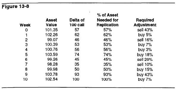
Feeding these inputs into a theoretical pricing model, we find that the call option which the hedger would like to own has a delta of 57. This means that if the hedger actually owned the call (instead of owning the underlying asset together with a 100 put) in theory he would have a position equivalent to owning 57% of his asset. Therefore, if he wants to replicate the combination of the underlying asset and the 100 put, he must sell off 43% of his holdings in the asset. When he does that, he will have a position theoretically equivalent to owning a 100 call.

将这些输入参数放入理论定价模型中,我们发现该看涨期权的delta为57。这意味着,如果对冲者实际持有看涨期权(而不是持有标的资产和100看跌期权的组合),理论上他的仓位相当于持有其资产的57%。因此,如果他想复制标的资产加100看跌期权的组合,就需要卖出43%的资产持仓。这样,他的仓位理论上等同于持有一个100的看涨期权。

Now suppose a week passes and the value of his asset has risen to 102.26. What would be the delta of the 100 call which the hedger desires to own? Again, feeding all the inputs into a theoretical pricing model, we find that the call now has a delta of 62. If the hedger wants a position which is equivalent to a long call, he now needs to own 62% of his original holding in the underlying asset. He must therefore buy back 5% of his original holding in the asset.

假设一周后,资产价格上升至102.26。这时,对冲者想要持有的100看涨期权的delta会是多少?再次将所有参数输入理论定价模型,我们发现此时该看涨期权的delta变为62。如果对冲者想获得与看涨期权相等的仓位,现在他需要持有原始资产持仓的62%,因此必须回购5%的资产。

Suppose another week passes and the value of the asset has fallen to 99.07. Using the new market conditions, the 100 call would now have a delta of 46. In order to replicate the call position, the hedger must now sell off 10% of the asset, so that he owns only 46% of his original holding.

再假设一周后,资产价格下降到99.07。根据新的市场情况,100看涨期权的delta变为46。为了复制该看涨期权的头寸,对冲者现在需卖出10%的资产,使其仅持有原始持仓的46%。

Notice what the hedger is doing. He is periodically rehedging his original holding to create a position with the same delta characteristics as the call. If he continues to do this over the ten-week period, he has, in effect, created a ten-week call at an exercise price of 100.

观察对冲者的操作,他在定期调整持仓以创建与看涨期权delta特征相同的头寸。如果他在整个十周期间持续这样做,就等效于创建了一个行权价为100、到期为十周的看涨期权。

The reader may have already realized that we are simply repeating the example in Figure 5-1, but in a slightly different form. In that example, we purchased an underpriced call and replicated the sale of the same call through a continuous rehedging process. In our current example we are also replicating the call through a continuous rehedging process. But here we want to purchase the call rather than sell it. All our adjustments are therefore the opposite of those in Figure 5-1. Note also that at week ten (expiration), instead of liquidating the position, as we did in Figure 5-1, we plan to buy in the remainder of the asset. It was always our intention to retain our entire holding of the asset at expiration. The replicated position in our current example is shown in Figure 13-8.

读者可能已注意到,这与图5-1的例子相似,只是形式稍有不同。在该例子中,我们购买了一个低估的看涨期权,并通过连续对冲过程来复制卖出同样的看涨期权。在当前例子中,我们也通过连续对冲复制了看涨期权,但这里我们是要买入该看涨期权。因此,我们的所有调整与图5-1中的相反。另外,在第十周(到期日),我们计划买回剩余的资产,而不是像图5-1那样平仓。我们的初衷就是在到期时保留整个资产持仓。此复制头寸在图13-8中展示。


In order to replicate the call, the hedger will have to buy back some of the asset when the market rises and sell some of the asset when the market falls. The unfavorable adjustments (buying high, selling low) suggests that there will be a cost associated with this rehedging process. What will the cost be? If the replication process offers the same protection as owning a 100 put, then one might expect the cost of the replication process to be the same as the theoretical value of the ten week 100 put. This is indeed the case. Using the previously listed inputs, the Black-Scholes model yields a theoretical value for the 100 put of 2.55. This is identical to the cost of the replication process described in Figure 13-8.

为了复制看涨期权,对冲者在市场上涨时需回购部分资产,在市场下跌时需卖出部分资产。这种“高买低卖”的不利调整意味着再对冲过程中会产生一定成本。这个成本是多少?如果复制过程能提供与拥有100看跌期权相同的保护,那么可以预期其成本等同于该期权的理论价值。确实如此,使用前述参数,Black-Scholes模型计算出的100看跌期权理论价值为2.55,与图13-8中的复制过程成本相同。

The rehedging process is an attempt to replicate the automatic rehedging characteristics of the option. As a hedge against an underlying position, an option has the very desirable characteristic of offering greater protection as the market moves adversely, and less protection as the market moves favorably. In effect, the option automatically rehedges itself to fit the required amount of protection. This is the influence of the gamma on the option's delta. When a hedger attempts to replicate the characteristics of an option by continuously rehedging the underlying position himself, he is simply trying to replicate the automatic rehedging (gamma) characteristics of the option. The cost of the option, or the cost of the rehedging process, is the price the hedger pays for the option's gamma characteristics.

再对冲过程试图复制期权自动再对冲的特性。作为标的头寸的对冲工具,期权在市场不利时提供更大保护,市场有利时减少保护,这就是期权gamma对delta的影响。对冲者通过不断对冲标的头寸来模拟期权的特性,即试图复制期权的自动再对冲(gamma)特性。期权的成本或再对冲的成本即对冲者为期权gamma特性支付的价格。

Since we need to continuously compute the delta to replicate an option through a rehedging process, this method of replication requires us to use a theoretical pricing model. We are therefore likely to encounter many of the same problems which we encounter anytime we use a theoretical pricing model to evaluate an option. Is the model itself correct? Do we have the right inputs? Leaving aside the question of the model's correctness, anyone wishing to use this method will have to come up with a reasonable volatility estimate. If the volatility estimate turns out to be too high or too low, the cost of replicating the option will be more or less than originally expected. But notice that the cost of replication will always be the right cost. If the market is more volatile than expected, the cost will be greater in terms of required adjustments. But the value of the option would also have been greater. Higher volatility means a higher theoretical value. In the same way, if the market is less volatile than expected, the cost will be less in terms of required adjustments. The value of the option would also have been less. Lower volatility means a lower theoretical value.

由于需要持续计算delta来再对冲以复制期权,该复制方法要求使用理论定价模型,因此可能遇到使用理论模型时常见的问题:模型是否正确?输入是否合适?撇开模型正确性不谈,使用该方法的人需提供合理的波动率估计。如果波动率估计过高或过低,复制期权的成本也会相应多或少。但复制成本总是反映市场实际情况。如果市场比预期更为波动,调整成本会更高,但期权的价值也会更高;反之,市场波动较低时,调整成本较低,期权价值也会相应降低。

This process of continuously rehedging an underlying position to replicate an option position is often referred to as portfolio insurance. The method can be used to protect any long or short position against adverse movement, but it is most commonly used by fund managers who wish to insure the value of the securities in a portfolio against a drop in value. For example, suppose a manager has a portfolio of securities currently valued at $100 million. If he wants to insure the value of the portfolio against a drop in value below $90 million, he can either buy a $90 million put, or he can replicate the characteristics of a $90 million call. If he is unable to find someone willing to sell him a $90 million put, he can evaluate the characteristics of the $90 million call and continuously buy or sell the portion of his portfolio required to replicate the call position. In effect, he has created his own put.

这种通过持续再对冲标的头寸来复制期权的过程常称为投资组合保险。该方法可用于保护多头或空头头寸免受不利变动的影响,尤其常用于基金经理保护证券组合的价值。例如,假设某经理的组合价值为1亿美元,若他想保护其价值不低于9000万美元,可以选择购买9000万美元的看跌期权,或复制9000万美元的看涨期权特性。如果无人愿意卖出9000万美元的看跌期权,他可以评估9000万美元的看涨期权特性,持续买卖组合中的部分持仓以复制该看涨期权的头寸,实质上创造了一个看跌期权。

Unfortunately, the costs of buying and selling a large number of securities in odd amounts may be quite high. While the concept of portfolio insurance may be attractive from a theoretical perspective, the transaction costs may make the process too expensive to be of practical value. Is there any way a fund manager can use portfolio insurance while keeping transaction costs within acceptable bounds? One common method involves using futures contracts as a substitute for the portfolio holding. If the mix of securities in a portfolio approximates an index, and futures contracts are available on that index, the manager can approximate the results of portfolio insurance by purchasing or selling futures contracts to increase or decrease the holdings in his portfolio. In the United States several index futures are available, the most popular being the futures contract on the S&p 500 index traded at the Chicago Mercantile Exchange. Many fund managers use S&P 500 futures to insure their portfolios against adverse movement in the stock market. This method is not without risk, since the S&p 500 index is unlikely to exactly duplicate the holdings of any one portfolio. Still, the risk may be acceptable given the reduced transaction costs.

遗憾的是,不规则数量的大量证券买卖成本可能较高。虽然理论上投资组合保险的概念很吸引人,但交易成本可能过高而难以实际操作。那么基金经理是否有办法在控制交易成本的前提下使用投资组合保险?一种常见的方法是用期货合约替代部分组合持仓。如果组合中的证券与某指数相近,且该指数的期货合约可用,经理可以通过买卖期货来调整持仓,从而接近投资组合保险的效果。在美国,有多种指数期货可供选择,其中最受欢迎的是在芝加哥商品交易所交易的标普500指数期货。许多基金经理使用标普500期货来对冲股票市场的下跌风险。这种方法并非没有风险,因为标普500指数不太可能与任何单个组合完全一致,但在降低交易成本的情况下风险可能是可接受的。

Even if options are available on an underlying asset, a hedger may still choose to effect a portfolio insurance strategy himself rather then purchasing the option in the marketplace. For one thing, he may consider the option too expensive. If he believes the option is theoretically overpriced, in the long run it will be cheaper to continuously rehedge the portfolio. Or he may find insufficient liquidity in the option market to absorb the number of option contracts he needs to hedge his position. Finally, the expiration of options which are available may not exactly correspond to the period over which he wants to protect his position. If an option is available, but expires earlier than desired, the hedger might still choose to purchase options in the marketplace, and then pursue a portfolio insurance strategy over the period following the option's expiration. For all these reasons, portfolio insurance has become an increasingly popular method of protecting a position in an underlying asset.

即使标的资产的期权可用,对冲者仍可能选择自行进行投资组合保险,而非直接购买市场期权。一方面,他可能认为期权价格过高;若认为期权被高估,长期来看持续再对冲更便宜。另一方面,期权市场可能流动性不足,难以吸收其需要的数量。此外,可用的期权到期时间可能与其需要保护的周期不完全匹配。若期权的到期时间早于预期,对冲者仍可选择在市场上购买期权,在期权到期后继续采取投资组合保险策略。由于这些原因,投资组合保险已成为保护标的资产头寸的热门方法。